CMA-ES Source Code
This page provides implementations of the CMA-ES and links to libraries that contain such implementations. All implementations provided in this page follow very closely Hansen (2006). They
support small and large population sizes, the latter by implementing
the rank-µ-update (Hansen et al, 2003) with
non-uniform recombination weights (Hansen and Kern,
2004) and an improved parameter setting for the step-size
adaptation (Hansen and
Kern, 2004). The default population size is small (Hansen and Ostermeier,
2001). Further (optionally) supported features:
- All implementations, except for the minimalistic codes for
reading, provide an independent restart procedure with increasing
population size (Auger
and Hansen, 2005) and standardized data output for
visualization.
- All implementations, except for the minimalistic code
for reading, optionally support a "separable/diagonal"
initial phase, where the covariance matrix remains diagonal (Ros and Hansen, 2008). The
latter permits a faster learning of the diagonal elements and reduces the internal time complexity from quadratic to linear
which might be useful for dimensionalities, say, larger than a hundred.
- Matlab since version 3.0 and Python since version 0.9.92 support an additional uncertainty handling (Hansen et al, 2009, set option
Noise.on='yes', however, don't rely on this option without a rough
understanding of what it does).
- Matlab since version 3.40.beta and Python since version 0.9.92 implement the idea of active CMA (Jastrebski and Arnold, 2006, see option CMA.active or CMA_active), where a "negative" covariance matrix update explicitly reduces the variance in directions where bad samples were found. The implementations differ and also deviate considerably from the original paper.
- Python since version 0.9.92 implements selective mirrored sampling (Auger et al, 2011), where a few of the worst solutions are mirrored.
Minimalistic code for reading and education is provided in Matlab/Octave and Python.
The specific formulation of a (real) optimization problem has a tremendous impact on the optimization performance. In particular, a reasonable parameter encoding is essential. All parameters should be rescaled such that they have
presumably similar sensitivity (this makes the identity as initial covariance matrix the right choice). Usually, the best approach is to write a wrapper around the objective function that transforms the parameters before the actual function call. The wrapper scales, for example, in each parameter/coordinate the value [0; 10] into the typical actual domain of the parameter/coordinate. To achieve this on-the-fly, a linear scaling of variables is provided in the Scilab and Python codes below. With this transformation, a typical initial sigma will be ≈ 2, see also below.
The natural encoding of (some of) the parameters can also be "logarithmic". That is, for a parameter that must always be positive, with a ratio between typical upper and lower value being larger than 100, we might use 10x instead of x to call the objective function. More specifically, to achieve the parameter range [10–4,10–1], we use 10–4×10³x/10 with x in [0; 10]. Again, the idea is to have similar sensitivity: this makes sense if we expect the change from 10–4 to 10–3 to have an impact similar to the change from 10–2 to 10–1. In order to avoid the problem that changes of very small values have too less an impact, an alternative is to choose 10–1 × (x/10)2 ≥ 0.
In the case where only a lower bound at zero is necessary, a simple and natural transformation is x2 × default_x, such that x=1 represents the default (or initial) value and x remains unbounded during optimization.
In summary, to map the values [0;10] into [a;b] we have the alternative transformations
-
a + (b-a) × x/10
-
a + (b-a) × (x/10)2 ≥ a
-
a × (b/a)x/10 ≥ 0 assuming that a > 0.
A simple way to achieve, for example, a lower bound a of a variable x is to use a + x2 instead of x in the objective function call (as already mentioned above). Lower and upper bounds a, b can be achieved with y = a + (b-a) × (1 – cos(π × x / 10)) / 2, where for 0 ≤ x ≤ 10 this is a strictly increasing bijective mapping into [a, b]. y remains between a and b also for any other value of x.
In the very same spirit, the boundary handling implemented in the C and Python codes uses a piecewise either linear or quadratic function to avoid numerical subtleties (however the implemented boundary handling does not shift the domain and therefore maps the domain center a + (b-a) / 2 to itself).
In any case, a reasonable (linear) scaling of variables in x should still be taken care of when the sizes of boundary intervals and the (supposed) sensitivities do not agree. Variables that consistently end up on the (same) boundary can be removed. The Python and Scilab codes provide the means to (tentatively) remove variables from the optimization.
Another reasonably good method for handling boundaries (box-constraints) in connection with CMA-ES is described in A Method for Handling Uncertainty in Evolutionary Optimization...(2009) (pdf), see the prepended Addendum and Section IV B. In this method, a penalty, which is a quadratic function of the distance to the feasible domain with adaptive penalty weights, is implemented in Matlab and Python codes below.
Addressing non-linear constraints is more intricate. In benign cases the optimum is not very close to the constraint and simple resampling works fine. The provided implementations do automated resampling when the objective function returns NaN. A simple (to implement) alterative is to compute Σi (xi - domain_middlei)2 + a_large_constant as objective function value for infeasible solutions. This might often work better than resampling. Yet, it still might work poorly if the optimum is at the domain boundary.
The class cma.ConstrainedFitnessAL
provides a non-linear constraints handling which works well when the optimum is at the boundary given the function is sufficiently smooth.
For a very short and general overview on boundary and constraints handling (as of 2014 not anymore up-to-date though) in connection with CMA-ES, see the appendix of The CMA Evolution Strategy: A Tutorial, p.34f.
After the encoding of variables, see above, the initial solution point x0 and the initial standard deviation (step-size) σ0 must be chosen. In a practical application, one often wants to start by trying to improve a given solution locally. In this case we choose a rather small σ0 (say in [0.001, 0.1], given the x-values "live" in [0,10]). Thereby we can also check, whether the initial solution is possibly a local optimum. When a global optimum is sought-after on rugged or multimodal landscapes, σ0 should be chosen such that the global optimum or final desirable location (or at least some of its domain of attraction)
is expected not to be (far) outside of x0 ± 2σ0 in each coordinate. (Remark that in Rn, if each boundary domain is in distance σ, then the boundary corner is σ √n away, which poses a slight dilemma for larger n.)
The source code from this page writes output data that can be plotted either with the respective code or with the following stand-alone versions (the data formats are largely inter-compatible):
The plotted output files must be in the current folder. See sections Example Output and Testing Code and More Examples for examples of the resulting output.
CMA-ES/c-cmaes on GitHub
(download zip file)
provides a pure ANSI C
implementation in a fairly object-oriented way, where the iteration
step can be explicitly controlled. Also several independent optimization instances can be used at the same time. Therefore, the integration into any existing program in C or C++, should be fairly easy. The option "diagonalCovarianceMatrix" does not provide linear space complexity.
A few libraries implement the CMA-ES in C++:
The pCMALib parallel library in FORTRAN 90.
A Java version is provided, where originally the core procedures from the ANSI C version were
used:
Also the following libraries implement the CMA-ES in Java.
Code for Reading
purecmaes.m is a
minimalistic implementation running in Matlab and
Octave. It is mainly provided for educational purpose: reading, understanding
and running basic experiments. It contains roughly 100 lines, with 20 lines
reflecting the core implementation of the algorithm. This implementation has
only rudimentary termination conditions implemented, under some circumstances
it might be numerically inefficient and it should probably not be used for
running "real" experiments.
Production Code
cmaes.m
(version >3.60) provides an
interface similar to Matlab's optimization routines, e.g. fminsearch
and fminunc. The following (optional) variants/extensions are implemented.
- option LBounds and UBounds: coordinate wise boundary handling (Hansen et al, 2009)
- option Noise.on: uncertainty (noise) handling (Hansen et al, 2009)
- option CMA.active: a substractive update of the covariance matrix, similar to Jastrebski and Arnold (2006) (set option CMA.active = 1 with check for positive definiteness or CMA.active = 2 without checking). This version might become the default in near future.
- option DiagonalOnly: only the diagonal of the
covariance matrix is adapted for a number of initial iterations (Ros
and Hansen, 2008) which leads to a faster learning of a variable scaling and also reduces the internal time complexity of the algorithm from quadratic to linear (meanwhile no correlations are learned)
The
verbosity options have been rectified as Disp Log and Save options.
By default (LogModulo=1), output data is written to files
(ASCII) and plotcmaesdat.m is a stand
alone function to plots these data. The function can be used to
investigate the output data from cmaes.m while the optimization is
running. Under Octave plotcmaesdat.m works since Version 3,
for earlier versions option LogPlot of cmaes.m must be set to zero
(package octave-forge is needed in any case).
cmaes3.33.integer.m is an experimental
version for variables with given granularity (e.g. mixed-integer) via option StairWidths,
see also A CMA-ES for Mixed-Integer Nonlinear Optimization.
cmaesV255.m (version 2.55, July 2007) is
the former version which saves the data record history internally. plotcmaes.m and dispcmaes.m are stand alone functions to
plot/display data output from cmaes.m before version 3. They can be
used to investigate the output data while the
optimization is still running.
For Octave the package octave-forge is needed (thanks to
Luís Correia for the advise).
pycma is a production code with a functional interface cma.fmin2() and the class cma.CMAEvolutionStrategy with ask-and-tell interface (see Collette et al 2010 and below). An improved boundary handling is implemented and many more features that are useful in practice: a variety of termination and verbosity options, variable scaling, variable masking...
- Installation of the latest release from PyPI/cma
at the Python Package Index:
- type "
pip -U install cma" in a command shell (be aware that you might have several Python distributions, each of them providing their own pip command)
- API documentation
- Source code at github
- Source code and docs for version 1.x (single file)
This (single-file) module works with Python 2.6, 2.7 (recommended) and 3.x
(little tested). CAVEAT: the interface of
fmin and
OOOptimizer.optimize has changed since version 1.0.
If necessary, download the last version 0.92.06 of cma.py with the
old interface.
The pycma module includes cma.purecma (API epy-docs with source code), a shorter implementation for reading and education.
cma.purecma can be used from a stand alone file and has a minimal number of dependencies, in particular it does not need the python module numpy. For this reason it is slower (however it runs with very competitive speed in pypy, a Python with just in time compilation). If the Python module matplotlib is available, basic plots are provided.
[EDIT 2024] Installing (a recent) Python using conda, by creating a new python environment/installation (downloading ~140MB), named py312, and activating the environment in the current shell and installing the pycma package:
    conda create --name py312 python=3.12 scipy matplotlib jupyter ipython pandas scikit-learn
    conda activate py312
    pip install cma
Python is (arguably) the
most popular
well-designed, general purpose, object-oriented scripting programming language. Python is available on almost every computer (since many years), and provides, based on the numpy package, an excellent (and free) environment for scientific computing (since not so many years). In particular the powerful ipython shell (also in combination with the Jupyter notebook) provides a superset of the python shell and allows, for example, to easily access the functionality of matplotlib with MATLAB/Octave-style interface (via the %pylab mode). Three distributions provide an easy installation of all necessary (and many more useful) tools, including ipython:
- Anaconda
(download here)
is a comparatively light-weight cross-platform distribution which does not interfere with other already installed Python versions (other than prepending to the system path).
- Enthought Canopy, download here (for Mac/Windows only the free 32-bit version does not require registration), not only but in particular on non-Linux systems.
- Sage, which is entirely open source (
sage -ipython), with additional emphasis on symbolic computation and some sage-only functionality. For general infos see the Sage documentation, for a possibly useful install info see sage-matlab.
For a more comprehensive list of re-packaged Python distributions see for example here.
For more information on IDEs see for example here.
Integer versus true division
Update (2016): An excellent and comprehensive resource on how to go about the Python 2/3 dilemma can be found here.
In Python, the "//" operator denotes truncated division. One of the biggest design mistakes in Python versions ≤ 2.x is the division operator "/". The operator behaves depending on the type of the operands: integer, 1/2 == 0, or float, 1./2 == 0.5, division. This weird and bug-prone behavior, inherited from C, has been abandoned from version 3 and can fortunately also be changed in previous versions: to get the "new" ("true") division where 1/2 == 0.5 in Python 2.x, we can use python -Qnew instead of python (however this is depreciated), or type
from __future__ import division
at the (i)python shell right after startup. The same can be used as first line in a python script or module. To change the default behavior of ipython run ipython profile create in the OS-shell to create a profile and add
c.InteractiveShellApp.exec_lines = ['from __future__ import division']
in the file ~/.ipython/profile_default/ipython_config.py (the line is already half prepared, commented). I also add from __future__ import print_function thereby enabling the print function (available since Python version 2.6, default from version 3.0) replacing the print statement (default before version 3.0).
OS X 10.9 (Mavericks)
Under OS X 10.9 one might observe (very) sluggish behavior in a python shell. This is due to App Nap (putting apps to sleep to save energy) and can be resolved using the appnope package.
Two interfaces are provided. An object oriented
ask-and-tell interface (cma_new etc.), where the loop
control remains with the user, and a functional interface (cma_optim).
An example output from a run of CMA-ES on the 12-dimensional
Rosenbrock function, using python "import cma; cma.plot()" for plotting
(having installed Python and pycma).
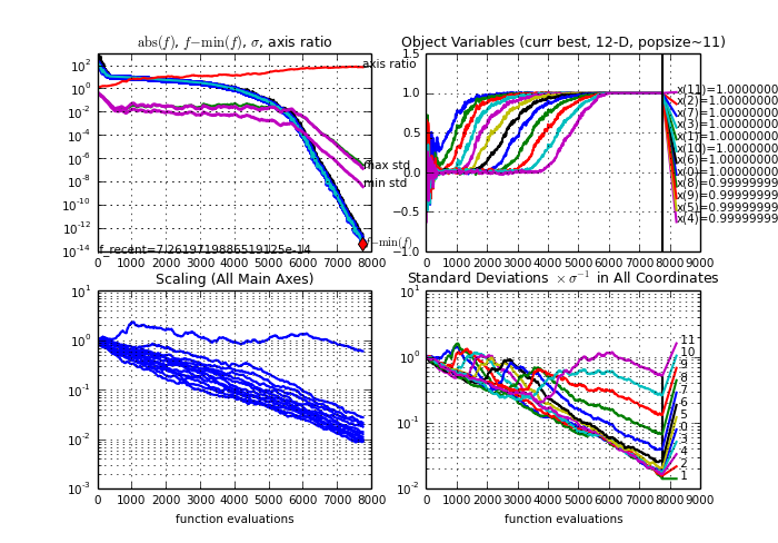
The lower figures show the square root of eigenvalues (left) and of
diagonal elements (right) of the covariance matrix C. The actual sample
distribution has the covariance matrix σ2 C. Weights
for the covariance matrix are set proportional to w_k = log((λ+1)/2) - log(k) for k=1,...,λ however with different learning rates for positive and negative weights.
The principle of the object-oriented ask-and-tell interface for optimization (see Collette et al 2010) is shown in the following abstract class in Python pseudocode (therefore untested).
class OOOptimizer(object):
def __init__(self, xstart, *more_args, **more_kwargs):
"""take an initial point to start with"""
self.xstart = xstart
self.iterations = 0
self.evaluations = 0
self.best_solution = BestSolution()
self.xcurrent = self.xstart[:]
self.initialize(*more_args, **more_kwargs)
def ask(self):
"""deliver (one ore more) candidate solution(s) in a list"""
raise NotImplementedError
def tell(self, solutions, function_values):
"""update internal state, prepare for next iteration"""
self.iterations += 1
self.evaluations += len(function_values)
ibest = function_values.index(min(function_values))
self.xcurrent[:] = solutions[ibest]
self.best_solution.update(solutions[ibest], function_values[ibest], self.evaluations)
def stop(self):
"""check whether termination is in order, prevent infinite loop"""
if self.evaluations > self.best_solution.get()[2] + 100:
return {'non-improving evaluations':100}
return {}
def result(self):
"""get best solution, e.g. (x, f, possibly_more)"""
return self.best_solution.get() + (self.iterations, self.xcurrent)
def optimize(self, objective_function, iterations=2000, args=()):
"""find minimizer of objective_function"""
iteration = 0
while not self.stop() and iteration < iterations:
iteration += 1
X = self.ask()
fitvals = [objective_function(x, *args) for x in X]
self.tell(X, fitvals)
return self
class BestSolution(object):
"""keeps track of the best solution"""
def __init__(self, x=None, f=None, evaluation=0):
self.x, self.f, self.evaluation = x, f, evaluation
def update(self, x, f, evaluations=None):
if self.f is None or f < self.f:
self.x, self.f, self.evaluation = x[:], f, evaluations
def get(self):
return self.x, self.f, self.evaluation
An implementation of an optimization class must (re-)implement at least the first three abstract methods of OOOptimizer: __init__, ask, tell. Here, only the interface to __init__ might change, depending on the derived class. An exception is pure random search, because it does not depend on the iteration and implements like
class PureRandomSearch(OOOptimizer):
    def ask(self):
        """delivers a single candidate solution in ask()[0],
           distributed with mean xstart and unit variance
        """
        import random
        return [[random.normalvariate(self.xstart[i], 1) for i in range(len(self.xstart))]]
The simplest use case is
res = PureRandomSearch(my_xstart).optimize(my_function)
A more typical implementation of an OOOptimizer subclass rewrites the following methods.
class CMAES(OOOptimizer):
    def __init__(self, xstart, sigma, popsize=10, maxiter=None):
        """initial point and sigma are mandatory, default popsize is 10"""
        ...
    def initialize(self):
        """(re-)set initial state"""
        ...
    def ask(self):
        """delivers popsize candidate solutions"""
        ...
    def tell(solutions, function_values):
        """update multivariate normal sample distribution for next iteration"""
        ...
    def stop(self):
        """check whether termination is in order, prevent infinite loop"""
        ...
A typical use case resembles the optimize method from above.
objectivefct = ...
optim_choice = 1
long_use_case = True
if optim_choice == 0:
optim = PureRandomSearch(xstart)
else:
optim = barecmaes2.CMAES(xstart, 1)
if long_use_case:
while not optim.stop():
X = optim.ask()
fitvals = [objectivefct(x) for x in X]
optim.tell(X, fitvals)
else:
optim.optimize(objectivefct)
print optim.result()
See the minimalistic Python code above for a fully working example.
Testing a stochastic algorithm is intricate, because the exact desired outcome is hard to determine and the algorithm
might be "robust" with respect to bugs. The code might run well on a few test functions despite a bug that might later compromise its performance. Additionally, the precise outcome depends on tiny details (as tiny as writing c+b+a instead of a+b+c can give slightly different values. The difference is irrelevant in almost all cases, but makes testing harder).
Comparing to a trusted code
An effective way of testing is to compare two codes one-to-one,
furnished with the same "random" numbers. One can use a simple
(random) number generator. The numbers need not to be normal,
but should be continuous and symmetric about zero. Tracking the internal state
variables for at least two iterations must lead to identical results (apart
from numerical effects that are usually in the order of
10-15). Internal state variables are the distribution mean,
the step-size and the covariance matrix, and furthermore the two
evolution paths.
Comparing to trusted output
For comparing outputs, at the minimum the fitness plots should be available.
The plots generated in purecmaes.m define a more
comprehensive set of reasonable output variables: fitness, sigma,
sqrt(eigenvalues(C)), xmean.
The code should be tested on the following objective/fitness functions that can be found, for
example, in purecmaes.m, and the results
should be compared to trusted output, e.g. the one below ☺ The default test case can be 10-D.
Besides the default population size, it is advisable to test also with a much larger population size, e.g. 10 times dimension. I usually use the following functions, more or less in this order. If not stated otherwise, we assume X0=0.1*ones and sigma0=0.1 in 10-D and default parameters.
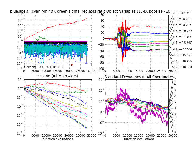
- On a random
objective function frand (e.g. f(x) is uniform in [0,1] and
independent of its input x). Step-size σ and the eigenvalues of
C should be tracked and plotted. log(σ) must conduct a symmetric
(unbiased) random walk. The iteration-wise sorted log(eigenvalues) will slowly
drift apart, quite symmetrically but with the overall tendency to
decrease. Eventually, the condition number of C will exceed numerically
feasible limits (say 1e14, that is, axis ratio 1e7), which should be covered in the code as termination
criterion.
Random function
|
- The sphere function fsphere
- it takes between 1000 and 1200 function evaluations to reach function value 1e-9
- with sigma0=1e-4, it takes about 300 additional function evaluations to increase sigma at the beginning to a reasonable value, see the green line in the upper left subplot. This test can "replace" the essential test of a search algorithm on a linear function (e.g. f(x) = x(1)).
Sphere function
|
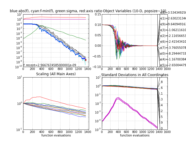
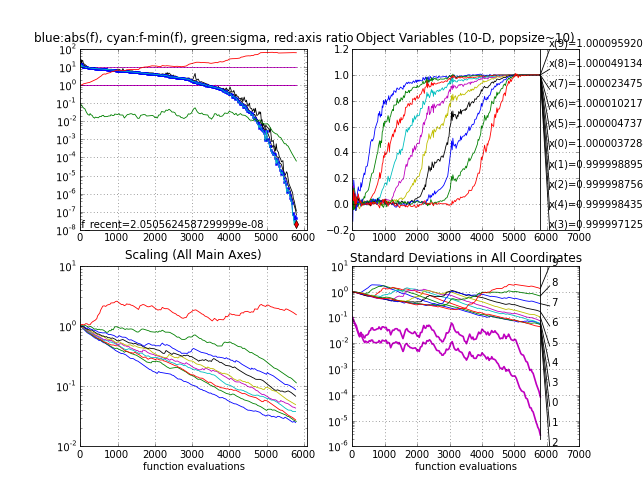
- The Ellipsoid felli, where it takes between 5000 and 6000 function evaluations to reach function value 1e-8. The
eigenvalues (Scaling plot) get a nice regular configuration on this function. Note that both subplots to the left are invariant under any rigid transformation of the search space (including a rotation) if the initial point is transformed accordingly. This makes a rotated Ellipsoid another excellent test case.
Ellipsoid function
|
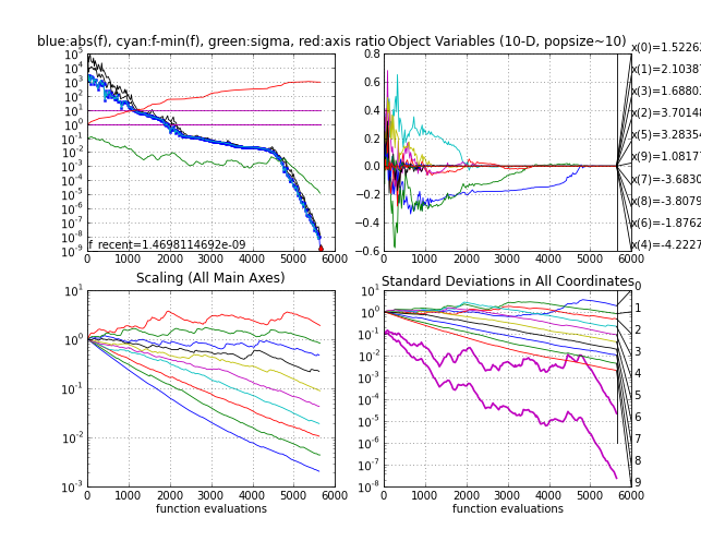
-
The Rosenbrock function frosen, the first non-separable test case where the variables are not independent. It takes between 5000 and 6000 function evaluations to reach a function value of 1e-8. With a larger initial step-size sigma0 in about 20% of the trials the local minimum will be discovered with a function value close under four.
Rosenbrock function
|
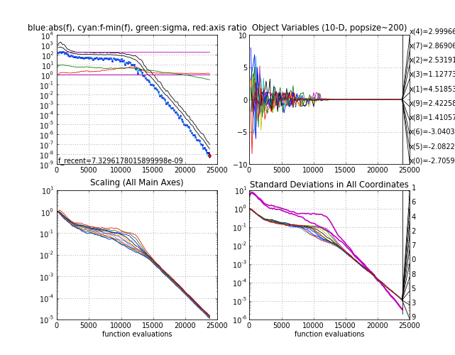
- The multimodal Rastrigin function. Here, X0 = 5*ones (the point 0.1*ones is in the attraction basin of the global optimum), sigma0 = 5 and population size 200. The success probability, i.e. the probability to reach the target f-value close to zero as in the below picture, is smaller than one and with smaller population sizes it becomes increasingly difficult to find the global optimum, see Hansen & Kern
2004.
Rastrigin function
|
- The Cigar fcigar.
Ideally, more dimensions should be tested, e.g. also 3 and 30, and different population sizes.
I appreciate any feedback regarding the provided source code and regarding
successful and unsuccessful applications or modifications of the
CMA-ES. Mail to  .
.
last change $Date: 2011-06-03 19:25:09 +0200 (Fri, 03 Jun 2011) $